Held–Karp TSP Visualizer
A Held–Karp TSP visualizer that uses realistic travel-time cost matrices.
Overview
I wanted a small, honest demo of what an exact TSP looks like when you use real travel times instead of straight-line distances. So I built a visualizer that runs the classic Held–Karp dynamic programming algorithm on a cost matrix sourced from road networks and traffic.
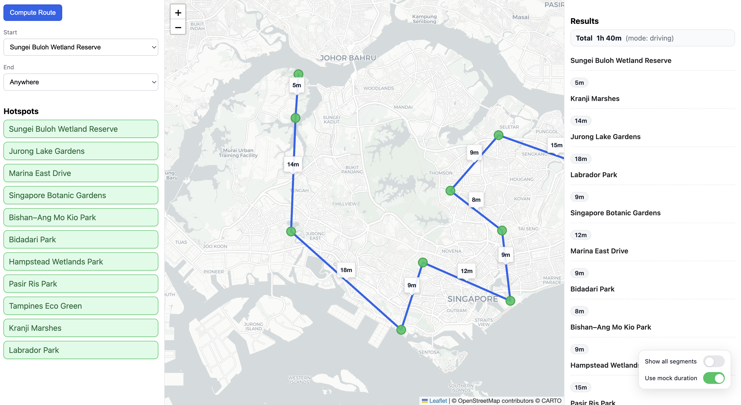
You pick points, it computes the optimal order, and it shows the route with the total travel time. No heuristics, no hand-waving—just a clear, step-by-step solution you can read and reason about.
The result is a ranked visit sequence and total travel time that reflect on-the-ground conditions.
Why Held–Karp?
Heuristics are fast and often good enough, but they can be opaque when you want to understand “why this order?” This project favors clarity over raw speed: Held–Karp is exponential, yet for small to medium sets it’s fast enough and provides ground truth you can compare against or use to benchmark heuristics.
Features
- Compute optimal visit order (minimize total travel time)
- Traffic-aware costs via distance matrix service
- Choose start/end points and include/exclude locations
- Visualize route order and total cost
- Server-side computation on Cloudflare Workers
Tech Stack
Frontend
- Next.js (App Router)
- TypeScript
- Tailwind CSS
Runtime & API
- Cloudflare Workers for server-side execution
- Distance Matrix API for realistic travel time/distance
How It Works
- Construct a pairwise travel-time cost matrix by batching distance matrix requests (details below), using driving mode with a specific departure time for traffic-aware durations.
- Run the Held–Karp dynamic programming algorithm on the matrix to compute the exact optimal route.
- Reconstruct the optimal visit order by backtracking predecessors from the DP table.
- Render the ordered sequence and total travel time in the UI.
This approach provides correctness (exact TSP on the given matrix) and realism (costs based on road networks and traffic).
Distance Matrix: Traffic-aware durations and batching
In plain terms: we ask the distance matrix service for travel times that reflect road networks and current or predicted traffic, then stitch the responses into a full N×N cost matrix.
- Traffic-aware travel time: Request driving mode with a departure time to obtain traffic-informed durations (commonly surfaced as duration_in_traffic in responses).
- Request size limits: When requesting traffic-aware durations, per-request element limits apply. To fill an N × N matrix, split into N requests each with one origin and N destinations (or chunk destinations further) so each request stays under the element cap.
- Aggregation: Combine all batched responses to assemble the full cost matrix, cache results, and proceed to optimization.
- Explicit configuration: Specify departure_time (for example, now) to enable traffic-aware calculations; without a departure_time, results are based on average time-independent traffic conditions.
- Prediction model: When using driving mode with a departure_time, you can further specify traffic_model (best_guess, optimistic, pessimistic) to influence how duration_in_traffic is predicted.
- Element limit detail: Requests that include departure_time with mode=driving are limited to a maximum of 100 elements per request; plan batching so each call remains under this cap.
Algorithm Details: Held–Karp DP
Intuition: think of DP[S, j] as “the cheapest way to start at s, visit exactly the nodes in S, and arrive at j.” We grow subsets one node at a time and always pick the best predecessor, then backtrack to recover the optimal order.
Held–Karp solves TSP exactly using dynamic programming over subsets:
-
State representation:
- Let n be the number of nodes and pick a start node s.
- Represent a subset S of nodes (including s) as a bitmask; a state is (S, j) meaning the best cost to start at s, visit all nodes in S, and finish at node j.
-
Base case:
- DP[{s}, s] = 0 and DP[{s}, j] = ∞ for j ≠ s.
-
Recurrence:
- For |S| ≥ 2 and j ∈ S, j ≠ s:
- DP[S, j] = min over i ∈ S \ {j} of (DP[S \ {j}, i] + cost[i][j]).
- Here cost[i][j] comes from the distance/time matrix (traffic-aware).
-
Tour closure (classic TSP):
- Optimal tour cost = min over j ≠ s of (DP[AllNodes, j] + cost[j][s]).
- Reconstruct the cycle by backtracking the chosen predecessors.
-
Open path (fixed start, free end):
- If you want a path from s that doesn’t need to return to s, use:
- Optimal path cost = min over j of DP[AllNodes, j].
- Backtracking reconstructs the path end j and the ordered sequence.
-
Complexity:
- Time: O(n^2 · 2^n) due to n · 2^n states and n transitions.
- Space: O(n · 2^n) to store DP states and predecessors for route reconstruction.
-
Practical notes:
- Use integer bitmasks for fast subset operations; index nodes 0..n-1.
- Precompute and cache cost[i][j] from the distance matrix service to avoid repeated calls.
- For small-to-medium n, Held–Karp is practical and yields a provably optimal route on the provided matrix.
- If constraints grow (e.g., time windows or very large n), consider heuristic/approximate methods layered on top of the same matrix.
Links
- Live Demo: TBA
- GitHub: https://github.com/fairy-pitta/hotspot_map
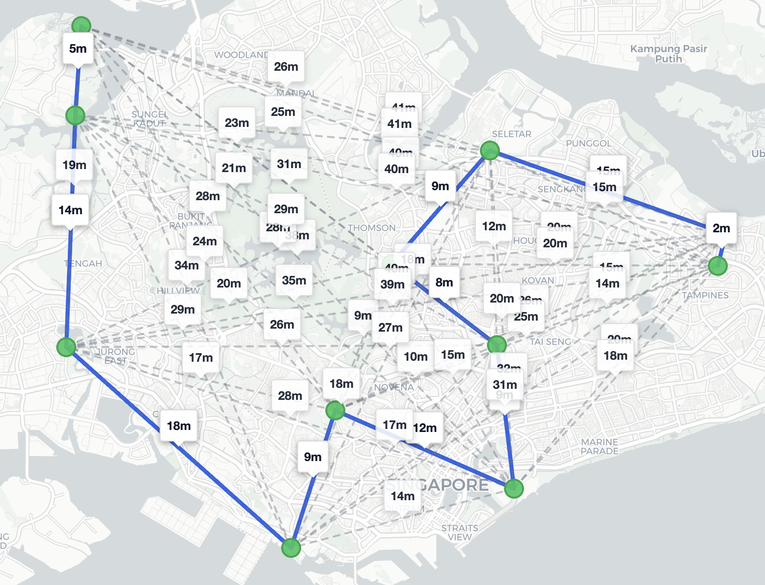
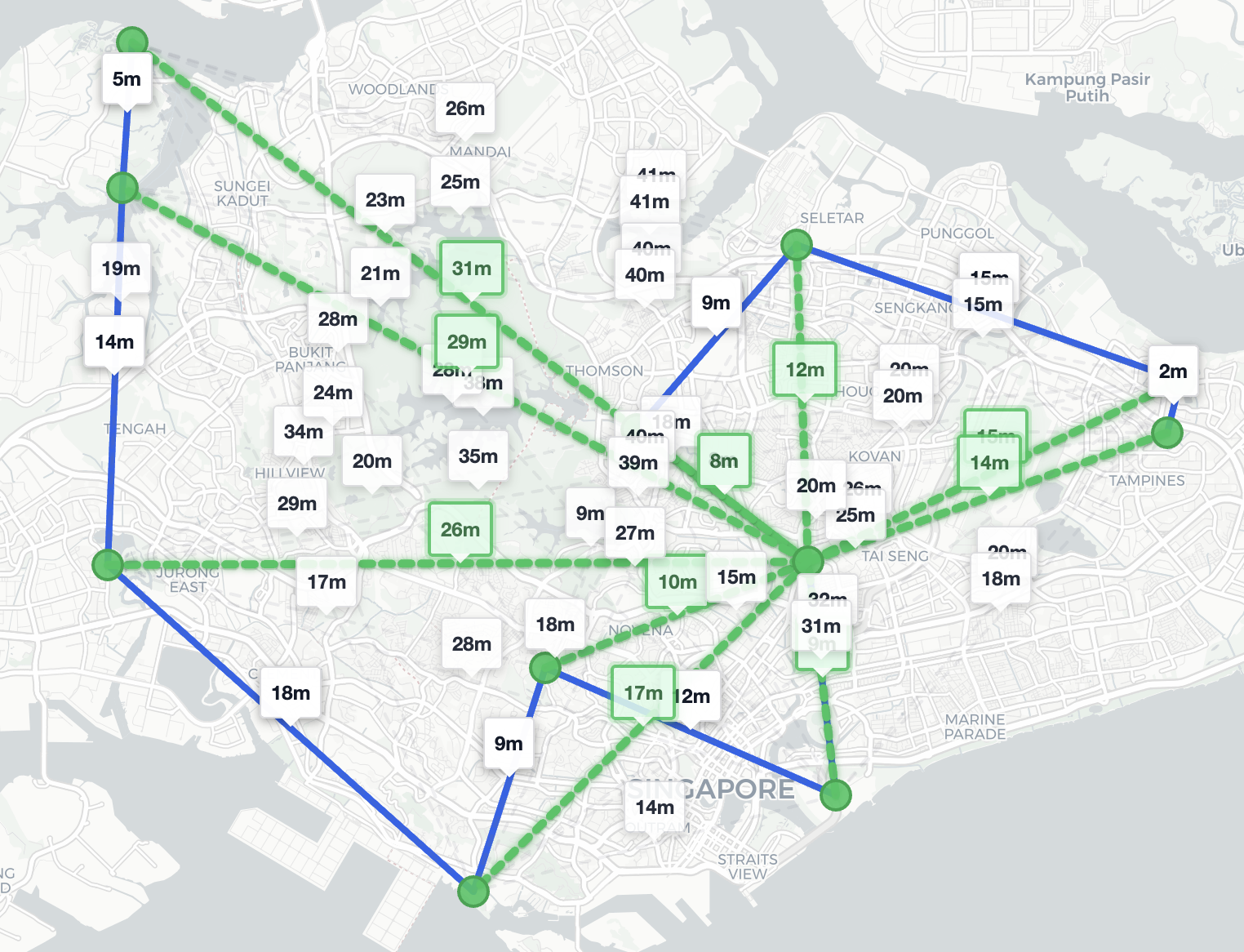
Gallery